Peter Masson, Bucknull & Masson
Abdul Sattar Babar, MEMRB-IRI
Worldwide Readership Research Symposium Valencia 2009 Session 1.4
Introduction
In the Spring of 2008 the Pakistan Advertisers Society (PAS) issued a call for tender for a survey that would was provide brand metrics (awareness and usage) directly related (‘single source’) to media exposure data for a wide range of digital and traditional media. It demanded a data delivery system that would enable the planning and evaluation of cross media schedules and provide, in reach and OTS terms, the effect of different budget allocations between media groups.
It was also to provide classification data that included a socio-cultural /lifestyle segmentation and a time audit of respondent’s work, social and media activities across the day.
The survey was to serve equally advertisers, media planners and media owners. It would represent at quantum leap from the currently available data which consisted of a one off National Readership Survey in 2007 and a small TV PeopleMeter panel in the three main metropolitan areas.
The project was awarded to MEMRB-IRI Pakistan based on a research design and delivery system developed in association with Bucknull & Masson/Sesame Systems Ltd. UK. This paper describes the design and execution of the study with particular reference to the media measurements designed to maximize cross media comparability.
The survey structure
The foundation of any media survey is the quality of the sample in terms of its design, response rate and size.
While the population of Pakistan is in the order of 165 million only around 30 million live in urban areas and it these that were to be represented in the survey universe. 20,000 interviews were to be conducted in two equal waves during March-May and September-November 2009. As many of the media to be measured were regional the sample was stratified by (15) major towns and all other towns within province and AB class homes oversampled by a factor of 2 with the disproportionate samples re- weighted at the analysis stage. Within each stratification a sample of homes was drawn (from detailed street maps) and individuals randomly selected from the household (using Kish tables). The sample was issued for interviewing in such a way as to create, as far as possible, an independent random sample day by day. This was important since we required to measure most media at the (average) day exposure level.
The interview was personal (pen and paper). There was no question of other forms of interviewing with very low fixed line telephone and internet penetration plus low literacy levels. In about 30% of the issued addresses no contact could be made and a substitute address issued. In only 1.5% of cases where contact was made was there a refusal. This extremely high response is related to the culture where one seeks to accommodate the needs of a visitor. The questionnaire was long (2 hours) and in some cases the interviewer would conduct it in two sessions at the respondent’s convenience.
Classification data
Apart from the usual demographics and Geographics three sets of data were required to meet the survey specification. These were Product and Brand metrics, Socio-cultural attitudes and daily Activities and feelings.
Product and Brand metrics
Product sectors were selected on the basis of their importance as advertising markets. In total 20 food sectors and 27 non food sectors were selected. (See Annex1)
Respondents were filtered in/out of the detailed sector questions on the basis of ‘do you eat/drink/consume/have in household/use’ product type xxxx?
Those passing the filter were asked to spontaneously name (Top of Mind (TOM)) the brands they were aware of in the sector. Then on the basis of a prompt list to name the Brand Used Most Often (BUMO) and brands sometimes used. Additionally questions were asked about responsibility for purchase decisions (a scale from’ I decide’ to ‘other family members decide’) and frequency of use of the product (times/volumes/expenditure per day/week/month as appropriate).
27
From the ‘BUMO’ and ‘sometimes use’ data interesting brand relationships can be visualized by plotting the proportion of BUMO (loyal users) as a proportion of total users (BUMO + sometimes users = brand penetration). An example of this graphic display of brand relationships can be seen in Annex 2.
Socio-cultural attitude statements
Prior to field work an extensive series of group discussions were conducted across the country insights from which formed the basis for the development of a battery of attitude statements (43) administered against a 5 point scale (strongly agree to strongly disagree). The 6 most discriminatory statements were:
| Table 1 | % agree |
| I like Western culture very much | 67.2 |
| I can’t spend even an hour without my mobile | 67.7 |
| My life is incomplete if without computer | 76 |
| I SMS/call friends till late at night | 68.6 |
| Marriages with the consent of parents are just right | 10.3 |
| I don’t want much change In my life | 11.2 |
| I see myself as religious | 11.4 |
From the full battery of statements 7 clusters were developed. As well as short text descriptions each segment was visualized with a long description for display in the software. Examples of the segments developed and their characteristics and visualizations can be found in Annex 3.
Activities and feelings
Respondents were asked to report, using a prompt list, WHERE they were (home, work etc.), WHAT they were doing (eating, praying etc.) and HOW they were feeling YESTERDAY by each hour of the day. The feelings were prompted as Pre-occupied with personal and work issues, stressed, angry, depressed, happy, calm/relaxed, tired or bored.
The software allows for the interlacing of WHERE and WHAT and WHAT and HOW (feelings). The data gives some considerable insights as to when and where consumers will be more receptive or less receptive to advertising messages. Some example results are given in Annex 4.
Overall these three areas of data, Product and Brand metrics, Socio-cultural attitudes and daily Activities and feelings coupled with basic demographics and Geographics provide the marketing and advertising planner with a very rich base from which to determine marketing and targeting strategies.
Media exposure
PAS wanted advertisers and planners to be able to plan holistically and evaluate in combination all the major media so that they could answer the question: ‘What would be the ‘effect’ of allocating different shares of the overall budget to different media groups’? ‘Effect’ was to be defined in terms of reach and OTS distribution. The media groups to be considered were newspapers, magazines, TV, radio, internet, SMS ads, cinema and outdoor.
Two key issues had to be addressed in the media questionnaire design.
First to provide a measure of OTS (opportunities to see) that had an equivalent meaning in terms of both Net AND Gross advertising exposure in each of the media. The definition1 aimed at as far as possible for media was ‘eyes/ears focused on the medium at the time the advertisement is on display’.
Second to allow for the time element in advertising ‘effect’. It is crucial in the evaluation of different cross media schedules that reach/OTS can be related to time periods (day by day and week by week). 20 OTS delivered in 2 days may be ‘over-kill’ but delivered over 2 months may be ‘under-kill’.
1 War of the Media Weights by Peter Callius, TNS-Sifo Sweden and Peter Masson, Bucknull & Masson UK, WRRS 2009 Valencia
Traditional probability models for estimating reach and frequency provide no evaluation of the time of exposure and the duplication estimates derived from the probability rely on an ‘assumption of independence’ between media events (simply not the case for TV, radio and Internet and in many cases not for newspapers2) and ignore the actual survey ‘single source’ duplication information.
The end result of the CMi media data collection should therefore be longitudinal diary/panel type data that would permit reach and frequency analysis at a level of week/day and time segment. The detail for each medium would be related to the time and space units in which the medium is bought and sold.
From a single interview (as CMi) respondents simply would not be able provide this reliably (by long term recall), nor were pen and paper diaries feasible due to literacy issues and there was certainly no budget to consider any ‘passive’ electronic devices. These in any case cannot cover (as yet) all the media we required.
We developed a limited set of questions which could be applied to all media ‘single source’ (except magazines and SMS) which provided a framework of data that enabled the modeling of a week of detailed behavior for each respondent at the average minute level day by day. This process is known as VDiary creation3.
The Sesame software model projects the data beyond the week so a planner can build and evaluate cross media schedules over any time period.
Where external ‘currency’ data exists the VDiary results from the ‘single source’ survey are normally calibrated to that ‘currency’ to avoid different results being available in the market. In this case in Pakistan no other data existed that was suitable to calibrate to.
The question framework
For each medium we start with a filter (in last month) and then a standard ‘Recency’ question. When was the last time you read title X, viewed channel Z ?
Yesterday, in last week, longer ago.
If respondent had read/viewed etc, in the last week…
On which specific days in the last week did you read/listen/view/browse? Mon/Tues/Wed/Thurs/Fri/Sat/Sun
These questions were applied to newspapers, TV, radio, Internet sites. They were also applied to cinema but the levels of cinema attendance were so limited we could not take cinema estimates to the day level. For outdoor we did not use this question but instead used the traditional frequency questions. On reflection it would have better to do so.
The question was how well would respondents be able to report their day of week behavior for the last week. The answer, which can be seen from the results in the following tables, was ‘quite well’ and certainly well enough for the VDiary modeling where the average of the day by day levels is always calibrated back to the yesterday ‘Recency’ (average day) claim.
Table 2
| Newspaper title | Dawn | Express | Khabrien | Nawa I Waqt |
| ‘000 | ‘000 | ‘000 | ‘000 | |
| Q. Day of week av.day
Q. ‘Recency’ Y’day (av day) |
181
192 |
1134
1140 |
323
354 |
635
646 |
| Q.Week with day of week Q ‘Recency’ Week recall | 440
440 |
2230
2230 |
807
807 |
1392
1392 |
All those that passed the week ‘Recency’ filter provided answers day by day. Their answers to a very limited extent underestimated their average daily reach when compared to the overall ‘Recency’ claim for yesterday (= average day)
2 Multi-Media Modelling by Dr. Paul Sumner and Peter Masson, Bucknull & Masson. (written paper for the WRRS, Boston, USA 2003)
3 A better alternative to Fusion: A modeling procedure to simulate independent media ‘currencies’ by Peter Masson and Paul Sumner, Bucknull & Masson, London (WM3 2006 Shanghai)
Table 3
| TV
channel |
Cartoon Network | Geo Ent. | Kashish | Ptv Home | Sony |
| ‘000 | ‘000 | ‘000 | ‘000 | ‘000 | |
| Q. Day of week av.day
Q. ‘Recency’ Y’day (av day) |
1541
1646 |
901
1039 |
655
600 |
2546
2519 |
1285
1484 |
| Q. Week with day of week Q ‘Recency’ Week recall | 2358
2558 |
1623
1858 |
898
994 |
3531
3942 |
2728
3221 |
For TV the day by day question was not as consistent with ‘Recency’ as for newspapers. Generally 10% of those passing the weekly ‘Recency’ questions failed to give a day by day claim (more in the case of Sony) and there was a notably lower estimate of the average day than provided by the ‘Recency’ claim.
From a modeling point of view this was not an issue. In the VDiary creation process the ‘Recency’ claims (day/week/month) are taken as the targets to be achieved. That is all those with a week ‘Recency’ claim will have at least one TV viewing event in the VDiary week. What the day by day data allows us to do is to establish a profile (proportion) of the known number week of viewers who are to be viewing on a particular day and a means to allocate specific individuals to particular days. If the actual number of day claims (say for Monday) fall under the target day total then more viewers who are in the week (but not already allocated) are selected (in proportion to their number of viewing days) for Monday to bring Monday viewers to the required level.
Table 4
| Radio stations | Fm 100 | Fm 101 | Fm 103 | Fm 106.2 | Fm 107 |
| ‘000 | ‘000 | ‘000 | ‘000 | ‘000 | |
| Q. Day of week av.day | 326 | 406 | 436 | 366 | 230 |
| Q. Y’day (av day) | 313 | 407 | 464 | 381 | 240 |
| Q. Week with day of week | 618 | 737 | 790 | 633 | 397 |
| Q. Week recall | 618 | 737 | 790 | 633 | 397 |
Table 5
| Internet sites | Yahoo | Gmail | Hotmail | Youtube | |
| ‘000 | ‘000 | ‘000 | ‘000 | ‘000 | |
| Q. Day of week av.day | 477 | 90 | 210 | 405 | 102 |
| Q. Y’day (av day) | 478 | 91 | 207 | 388 | 100 |
| Q. Week with day of week | 855 | 141 | 354 | 679 | 176 |
| Q. Week recall | 855 | 141 | 354 | 679 | 176 |
In both the cases of Radio and Internet all those passing the week ‘Recency’ claim gave a day by day answer. Their answers when averaged matched very closely to the yesterday (average) day ‘Recency’ claim.
We can only assume that the larger differences noted for TV are a result of the much longer list of channels involved and wider differences in frequency of viewing amongst TV channels than among radio. 76 TV channels were asked about compared 21 radio stations although only 53 TV channels and 11 radio stations are reported due to minimum sample size requirements.
Table 6
| Outdoor | Hoardings | Banner | Streamer | Posters | Bus/PTrans |
| ‘000 | ‘000 | ‘000 | ‘000 | ‘000 | |
| Q. Day of week av.day | 8324 | 10910 | 3128 | 10544 | 6257 |
| Q. Y’day (av day) | 5052 | 7422 | 1729 | 7306 | 3844 |
| Q. 1+ per week | 11881 | 14636 | 4908 | 14116 | 8966 |
| Q. Last Week ‘Recency’ | 10642 | 13741 | 4116 | 13084 | 8101 |
The frequency scale used for poster does not perform as well and results in notable overestimates for both day and week reach in relation to the ‘Recency’ claims. From a modeling point of view this again has little impact since it is the ‘Recency’ week question that determines who is eligible for a VDiary. While the allocation to the day is initially controlled by probability of
viewing in one day and will result in an over allocation it is then calibrated so that the average day equates to the yesterday ‘Recency’ claim. In this case respondents are discarded from each day, proportionately from each frequency group, so that the frequency profile is maintained for each day viewers.
Magazines cannot be handled in this way because the life of a title is much longer than the week and its full Last Issue Period reach (LIP) can take many weeks (if a weekly) and many months (if a monthly) to achieve. While experimental work has been conducted4 to develop a question sequence for an ad hoc survey more work is needed before implementing it. We relied therefore, regretfully, on the traditional ‘Recency’ and frequency probability model for magazines.
An evaluation of the VDiary results against ‘Recency’ results at the average day and week levels is shown below:
Table 7
| All pop | Age 12-24 | SEC A1,A2,B | ||||
| Sample/prfl | 10038 | 100 | 3608 | 35.9 | 3986 | 39.7 |
| Pop 000/prfl | 28504 | 100 | 10328 | 36.2 | 7938 | 27.8 |
| 000 | Week | Av Day | Week | Av Day | Week | Av Day |
| Dawn VDiary | 440 | 192 | 180 | 77 | 331 | 142 |
| Dawn ‘Recency’ | 440 | 192 | 180 | 73 | 331 | 145 |
| Cartoon Network VDiary | 2558 | 1667 | 1410 | 934 | 765 | 490 |
| Cartoon Network ‘Recency’ | 2558 | 1646 | 1410 | 952 | 765 | 510 |
| Fm 101 VDiary | 737 | 414 | 451 | 267 | 231 | 134 |
| Fm 101 ‘Recency’ | 737 | 407 | 451 | 269 | 231 | 134 |
| Yahoo VDiary | 855 | 480 | 495 | 280 | 549 | 315 |
| Yahoo ‘Recency’ | 855 | 478 | 495 | 274 | 549 | 301 |
The ‘Recency’ claims are used as the control for the VDiary (within gender, age, Social Economic Class and Province). How well the VDiary reproduces the average day and the week results is indicated in the table above for one vehicle from each of four media groups (Newspapers/TV/Radio/Internet). Results for more media vehicles can be found in Annex 5.
Day by day data
The reported reading/viewing etc. by day of week allows us to set controls in the VDiary creation to reproduce the day by day patterns. For smaller titles these day by day results (each day being based on one seventh to the sample) can be subject to random variation so we elected to create an average day to be applied to Monday to Thursday but separately for the Friday and Sunday holidays and Saturday where viewing and listening patterns are distinctly different. By creating a VDiary based on the day by day claims we are able to provide good estimates of the day by day accumulation where the cume of the 7 days will always match the weekly reach (‘Recency’ claim). This cume week reach cannot be relied on to match the week reach claim using probability models since reading/viewing etc. day by day are not necessarily independent events.
The following table gives a ‘count’ of the day by reach and cume across the week where it can be seen that the week VDiary cume matches the week ‘‘Recency’’ claim for all media groups (in Table 7).
Table 8
| Net Reach | |||||||
| ‘000’s | Mon | Tues | Wed | Thurs | Fri | Sat | Sun |
| Dawn
Dawn – cume |
216 | 216
294 |
216
342 |
216
363 |
90
378 |
171
399 |
218
440 |
| Cartoon Network Cartoon Net cume | 1711 | 1711
1998 |
1712
2205 |
1712
2356 |
1720
2477 |
1567
2524 |
1532
2558 |
| FM 101
FM101 – cume |
363 | 364
477 |
364
571 |
363
634 |
392
680 |
516
717 |
534
737 |
| Yahoo
Yahoo – cume |
520 | 520
634 |
520
704 |
519
750 |
382
767 |
525
825 |
374
855 |
4 Bringing magazines measurement into the 21st century : Daniëlle Siegers (CIM Belgium),
Patrick Hermie (Sanoma Magazines, Belgium), Peter Masson (Bucknull&Masson, London) (WM3 2008 Budapest)
Gross audience
Now in addition to estimates of Net audience it is also necessary (particularly in cross media comparisons) to have a comparable measure of Gross audience. Typically the Daily Press does not measure repeat ‘pick-ups’ during the day and is thus disadvantaged against media that typically do measure repeat exposure (particularly Internet and Posters). We asked the following question of people who read the title yesterday to determine the number of ‘pick ups’ per title on an average day.
Approximately how many times did you pick up the copy of XXXX for reading yesterday? Once, 2-3 times, 4-5 times, 6-7 times, 8-9 times, 10+ times
In table 9 below are some examples of the number of ‘pick-ups’ by title. In the Sesame schedule evaluation model they are treated in the same way as ‘Hits’ for Internet and the Gross Reach reported is the sum of the ‘pick-ups’ reported by each individual (* insertions). There is a notable degree of variation by title from 1.4 – 2.0 ‘pick-ups’ per issue.
Table 9
| Newspapers | Avg No.Pick- ups | % issue
read |
| Aaj | 2.02 | 66.9 |
| Awaz | 1.97 | 62.1 |
| Dawn | 1.73 | 64.0 |
| Express | 1.81 | 63.9 |
| Jang | 1.44 | 65.9 |
| Jurat | 1.62 | 65.7 |
| Kawish | 1.62 | 70.9 |
| Khabrien | 1.65 | 61.8 |
| Mashrik | 1.99 | 68.3 |
| Nawa I Waqt | 1.54 | 62.8 |
| Niya Akhbar | 1.57 | 61.0 |
| Qaumi Akhbar | 1.44 | 65.4 |
| The News | 1.52 | 70.2 |
We also asked the question as to the proportion of the issue read (all/almost all pages, more than half, about half and less than half). The differentiation between titles is relatively small from 61% to 70.2%.
In the Sesame data base every respondent is attributed a probability of passing an average page on the basis of this proportion of issue read claim (e.g. about half = 0.5). The planner may choose to use these average page probabilities or write in his own if, for example, (s)he is buying premium positions where the probability of passing the page will be much higher or decide not to use an ad. exposure factor at all.
Given that a factor is used the model reduces the chance of a single page being ‘passed’ but multiplies this chance by the number of ‘pick-ups’ since each gives a renewed opportunity of passing the page. So in the process the publisher may lose some net audience (although little on his premium front and back pages and Page 3) but will gain Gross audience from the multiple ‘pick- ups’. If the average page has 65% page traffic and the average number of pick up is 1.8 it would mean that the Gross reach would increase by 17% (and cpt reduced by 15%). For most titles therefore the model is likely to be advantageous to the publisher and it provides data at ‘level 3’ (if a full page is used) comparable to the television measurement level.
We believe this to be a significantly improved method of measuring and modeling daily newspaper reach and frequency.
Television and Radio.
The buying unit for TV and Radio (unlike the newspaper which is at the day level) is at the minute level. A measure of the audience is needed for the minute that the advertisement is aired.
So far in the VDiary creation we have only estimates for the Net (1+) audience at the day level. We need data to control the allocation of these Monday, Tuesday etc. audiences to broad day part segments and then to ¼ hours within segments.
We therefore asked all respondents (who viewed/listened yesterday) first at what broad (6 hour) time segments they viewed/listened to any channel yesterday. For each 6 hour period with listening/viewing claims the specific channels viewed/listened to were ascertained and then the specific ¼ hours these channel were viewed/listened to.
We also asked a generic question about TV Viewing and Radio listening (usually/sometimes/never) by weekday and each weekend day (Friday/Saturday/Sunday in Pakistan) by 3 hour periods across the day.
We are therefore in a position to allocate each respondent to day-parts and quarter hours across the day for the day that was the respondent’s yesterday. Using these yesterday claims as a proxy for his/her viewing on other days of the week we make the same day part allocation for that respondent on all other days of the week for which (s)he is a viewer. But in this process the reach level at each quarter is calibrated to match the yesterday ‘Recency’ claim day by day (with Monday to Thursday averaged) and, at the same time, respecting the usual times of TV viewing day reported in the generic TV viewing questions i.e. if the respondent claimed not to view TV at all on a Friday between 0600-0900 then (s)he would not be allocated to any station during this period in the day part allocation and calibration process.
Table 10
| 1/4 hr. Average day estimates | ||||||
| Geo News | Ptv home | Star Plus | ||||
| ‘000 | ‘Recency’ | VDiary | ‘Recency’ | VDiary | ‘Recency’ | VDiary |
| 09.00-09.15 | 337 | 325 | 73 | 75 | 142 | 145 |
| 09.15-09.30 | 298 | 289 | 57 | 59 | 129 | 132 |
| 12.00-12.15 | 321 | 319 | 52 | 53 | 325 | 318 |
| 12.15-12.30 | 318 | 314 | 65 | 68 | 358 | 356 |
| 19.00-19.15 | 1133 | 1087 | 356 | 327 | 1131 | 1135 |
| 19.15-19.30 | 1084 | 1047 | 387 | 355 | 1300 | 1298 |
| 22.00-22.15 | 1313 | 1268 | 300 | 279 | 1762 | 1676 |
| 22.15-22.30 | 1127 | 1102 | 222 | 218 | 1443 | 1394 |
Generally the ¼ hours level achieved are within +/- 5%. Sample size/weight unit is the limiting factor since adding or deleting one respondent/weight in the calibration will take the results over or under the target. The issue becomes greater within smaller demographic control cells. However we can make a further level of calibration at the average minute rating level which is the critical level for the calculation of Gross Reach.
Estimating ratings
To arrive at the average minute rating we must make an estimate of the number of minutes viewed/listened by each respondent in the ¼ hour. This can be implied from the data. If the respondent claims to view more than one station in the ¼ hour, the 15 minutes in the ¼ hour are divided equally between them i.e. if (s)he claimed to view/listen to 3 channels then each is attributed 5 minutes of viewing/ listening.
Further if the respondent did not claim to view/listen to the channel in both the preceding and following ¼ hours then (s)he is assumed to have entered or left the ¼ hour segment at the mid-point and is attributed 7.5 minutes viewing/listening. If (s)he viewed/listened to neither of the adjacent ¼ hours then (s)he is attributed 5 minutes. The following table shows the minute estimates and resulting ratings by quarter hour.
Table 13
| Segment | Geo News | Star Plus | ||||
| Net ‘000 | Avg Mins | Av rtg ‘000 | Net ‘000 | Avg Mins | Av rtg ‘000 | |
| 09:00-09:15 | 485.4 | 11.8 | 383 | 156 | 8.6 | 90 |
| 15:00-15:15 | 302.8 | 11.1 | 223 | 289.4 | 11.6 | 223 |
| 21:00-21:15 | 2353.8 | 12.2 | 1920 | 3046.6 | 12.4 | 2527 |
By combining the multiple channel viewing and the presence at adjacent quarters we arrive at a minutes viewed for each respondent by 1/4hr. Since this a fraction (of the 15 minutes available) we can adjust this fraction to account for any small calibration difference found at the ¼ hour level. Since this further adjustment/calibration is at an aggregate level we are not constrained by the size of the sample/weight value in matching the target level precisely.
What is important to remember however is that we are not trying to produce a ratings service but a basis for evaluating the reach and frequency of a schedule involving multiple spots where these small discrepancies will balance out.
Duplications
In a schedule evaluation not only must there be a good estimate of the Gross Reach but also of the Net Reach of combinations of channels across different time segments. The following table 11 shows the results for the duplicated reach from 3 channels (Geo New/PTV Home and Star Plus) for an average day and week and for an average day in the 0900-1200 and 1800-2100 segments. The results produced by the VDiary are entirely consistent with the ‘‘Recency’’ claims, all the VDiary estimates are within +/- 4% even within the demographic sub-groups.
Table 11
| Net Reach Geo News/PTVHome/Star Plus | ||||
| 000’s | Av. Day | week | Av day 0900-1200 | Av day 1800-2100 |
| All pop VDiary All pop ‘Recency’ | 15670
15294 |
19343
19347 |
1827
1763 |
9136
9180 |
| 12-24 VDiary
12-24 ‘Recency’ |
5727
5653 |
7146
7151 |
591
572 |
3396
3467 |
| AB VDiary AB ‘Recency’ | 4521
4494 |
5633
5634 |
530
554 |
2586
2675 |
Planners can therefore rely on VDiary schedule Reach and Frequency estimates with confidence. They provide a very good reflection of the original recall data while providing the capability of a full R&F analysis.
Internet
The Internet questions and the way they are handled in the VDiary model are exactly the same as for TV and Radio except that data was not collected at the ¼ hour level but only at the 6 hour day-part level. In order to provide estimates of Gross Reach (i.e. to include the multiple exposures during the 6 hour segment) we asked for both, time spent on the site and the number of separate visits made to the site.
These two measures (minutes spent and times visited (hits)) provide quite different estimate of Gross audience and a choice is required between them in relation to (level 3) comparability with other media. Comparisons are made between the two measures in the table 12 below:
Table 12
| 1 | 2 | 3 | 4 | 5 | 6 | 7 | 8 | 9 | 10 | 11 |
| 12.00-
18.00 |
Segment
Reach 000’s |
Avg No Visits | Average Minutes | Av. Mins per visit | Minutes as
% all segment minutes (360) |
rating based on
minutes 000’s |
Minutes Volume
Segment Gross |
Hits Volume
Segment Gross |
Index Volume
Gross Minutes |
Index Volume
Gross Hits |
| Yahoo Gmail Hotmail
Google Face Book Youtube |
478
91 207 388 67 100 |
2.761
2.394 1.918 3.621 1.974 2.708 |
18.47
14.8 21 20.13 20.12 17.18 |
6.7
6.2 10.9 5.6 10.2 6.3 |
0.051
0.041 0.058 0.056 0.056 0.048 |
24.5
3.7 12.1 21.7 3.7 4.8 |
8829
1347 4347 7810 1348 1718 |
1320
218 397 1405 132 271 |
100
15 49 88 15 19 |
100
17 30 106 10 21 |
Column 2 provides the Net Reach in the segment. Column 3 reports the average number of visits (by those visiting at all). Column 4 is the claimed number of minutes on site in the period (by those visiting at all).
The minutes spent can be translated via the proportion that they represent of the 360 minutes in the segment (col. 6) into an average minute rating (7) and then into a volume for the segment (8) (by multiplying up by 360). Equally volume can be created on the basis of Net Reach in the segment times the number of visits in the segment. Volume results are in columns 8 and 9.
While the rank order of sites for volume (Columns 10 and 11) is somewhat similar between minutes and ‘hits’ the absolute differences are substantial. Volume based on minutes is some 6-10 times higher than the visits volume. We therefore have to decide which should form the basis for the Gross measure.
The ‘minutes’ approach is predicated on the TV/radio model. If you are present during a minute in which the ad. is aired and if this was aired for 10 consecutive minutes then this would count as 10 OTS – although in fact it very likely that attention levels would fall dramatically through the period (a level 4 consideration). The difference on the Internet site measure is that while the ad. is presented for the (10) minutes it is not in a ‘solus’ position (as on TV) so it is very unlikely to on ‘clocking up ‘ an OTS each minute.
Equally we can compare with the Gross measure for outdoor where each passage past the site creates an OTS. If the person passed a site on the way to work and stood in view of it waiting for a bus for 5 minutes it still counts as only one passage and not that he glanced at it once every minute. Equally with the number of ‘pick-ups’ for print we do not take into account time spent reading on each ‘pick-up. Our decision therefore is to work with the ‘number of visits’ (hits) data as the most comparable Gross measure to other media.
The penetration of Internet is still very low in Pakistan and although we asked respondent to report on some 30 sites only the six sites shown in the charts above yielded a large enough sample size for publication of the results.
SMS advertising
The penetration of mobiles in urban Pakistan is 48% and it has now become a significant advertising medium with mobile owners receiving on average 5 SMS text/image ads. a week.
In effect this is electronic Direct Mail. Texts are ‘dropped’ onto X’000 mobiles via a Service Provider and controlled by geography (Province and Town).
To identify the reach and frequency of SMS contacts we need to know the Service Provider and billing type (Pre pay or monthly billing) and respondent’s Province and town – which we do from the classification data. What remains to establish is the likelihood of exposure when a text ad. hits his or her mobile. This was established by the following question:
How do you normally treat you advertising text messages? Delete without reading
See who it comes from and then delete if not relevant
Read/look at most text ads Read/look at all text ads
From this scale we established the probability of viewing a text ad.
We also asked some ‘qualitative question not used in the R&F model on whether texts were read immediately or batched and read later and whether they were generally found useful or not.
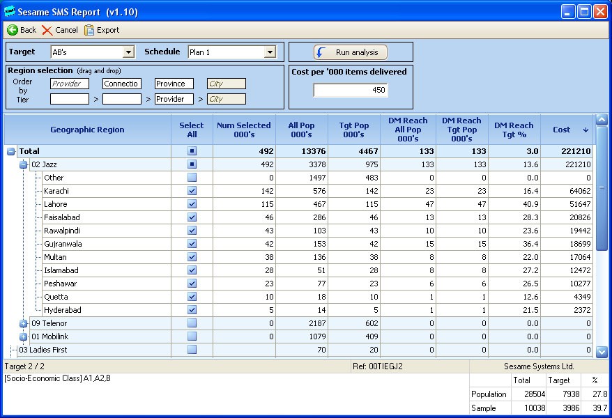
As can be seen in the following table the planner can select to work with a particular contractor (in this can Jazz). The ‘All Pop’ and the ‘Tgt.Pop’ columns show the total subscribers in ‘000’s for Jazz . In this case the planner has decided not to buy all 975,000 available target group AB’s but only 492,000, excluding subscribers in ‘other’ towns. This results in an AB Net reach of 133,000 (using the probability of viewing SMS text ad. data). This 133,000 represents a Net reach % of 13.6 of all Jazz AB subscribers and 3% of AB’s in urban Pakistan.
Once the planner has made his or her selection of Service Providers, towns and volumes this ‘schedule’ can be evaluated (including ‘multi-drop’ campaigns) alongside any of the other schedulable media or other SMS campaign selections.
Table 13
Outdoor
Traditional measures of outdoor involve a traffic survey (map aided recall/satellite tracking) and a site survey. The probability of the passage past each site can then be established and on the basis of the type of passage (on foot/driving car etc.) and the site characteristics (size, type, position, illumination) the probability of the site (ad.) being viewed. In some markets this data would be further modeled in relation to Census traffic flow data to compensate for limitations in the sample structure of the traffic survey.
Within the constraints of the CMi survey budget a separate/additional traffic survey was out of the question and the poster industry is not organized to readily provide the site survey. We could only therefore use a generic approach based on recall.
Respondents were presented with a series of images of outdoor (16) advertisements (e.g. Hoardings, Banners, Streamers, Digital screens etc.) and asked which they had seen (‘Recency’: yesterday, last week, last month) and how often they see them (frequency: daily, 5/6 days a week, 3-5 days a week, 1-2 days a week, less often) and for those who had viewed a particular type of site yesterday how many times they had seen such a site yesterday (1-5, 5-10, 11-20, 20+ times).
This is a virtually parallel set of questions to newspapers (apart from the specific days of the week) so that we are able to create a one week VDiary for outdoor in a similar manner.
In this process we created ‘outdoor buying vehicles’ based on the way they are bought. So we would have a vehicle for Karachi ‘banners’, or Lahore ‘digital sites’ and so on.
The data relates to the exposure to ALL such sites. The planner can write in a factor (in the software) to buy a proportion of the sites, based on the share of total inventory (site) that he is purchasing. This will require some care in making the judgment since the quality of sites (positioning/visibility) from different contractors will vary affecting the proportion of total R&F they will deliver. This is a very similar situation where overall cinema attendance is the measure.
The average daily and weekly reach and claimed daily ‘sightings’ was as follows:
Table 14
| Sample/prfl Pop 000/prfl | 10038
28504 |
100
100 |
Daily sightings | ||
| Wk ‘000 | %^ | AvDy 000 | AvD%^ | ||
| Kar-Billboards | 3400 | 11.9 | 1351 | 4.7 | 4.0 |
| Kar-Banner | 3131 | 11 | 1527 | 5.4 | 3.9 |
| Kar-Streamer | 1035 | 3.6 | 404 | 1.4 | 1.3 |
| Kar-Digital Screen | 1168 | 4.1 | 430 | 1.5 | 1.7 |
| Kar-Posters | 3278 | 11.5 | 1507 | 5.3 | 4.3 |
| Lah-Billboards | 1442 | 5.1 | 706 | 2.5 | 2.3 |
| Lah-Banner | 2154 | 7.6 | 1065 | 3.7 | 3.6 |
| Lah-Streamer | 844 | 3 | 381 | 1.3 | 1.5 |
| Lah-Digital Screen | 641 | 2.2 | 221 | 0.8 | 1.6 |
| Lah-Posters | 1634 | 5.7 | 791 | 2.8 | 3.7 |
| Raw-Billboards | 520 | 1.8 | 297 | 1 | 4.0 |
| Raw-Banner | 621 | 2.2 | 370 | 1.3 | 6.5 |
| Raw-Streamer | 336 | 1.2 | 178 | 0.6 | 4.3 |
| Raw-Digital Screen | 152 | 0.5 | 58 | 0.2 | 1.5 |
| Raw-Posters | 567 | 2 | 339 | 1.2 | 7.0 |
The weekly reach of billboards Karachi (6.330m.) is 53.7% and the weekly gross is (daily reach 1351* 4.0 sightings * 7 days = 37.822m.) giving an average OTS of 11.1 (37,822/3,400). In Lahore (3.739m) the weekly reach is 38.6% and the average OTS 7.9.
Cinema
We originally planned and collected data at the cinema complex level, usually there were not more than 2 per town and in most cases only one. We used our normal question formula of ‘Recency’ and days visited in the last week (without number of times per day as this would be a rare occurrence for cinema). However cinema penetration was very low indeed and the best that we could do was to establish a the probability of visiting a cinema in an average week within town
Media Gross and Net OTS comparability achievement
Table 15
| Vehicle | Ad page | Ad presence | attention to medium | Repeat Exposures
Included |
Net Reach
with 100 GRP |
| Level 1 | Level 2 | Level 3 | Level 4 | ||
| Newspapers | if page | implied
No No implied Part implied SMS ads. |
Yes | 21.1 | |
| Magazines | No | 14.7 | |||
| TV | Not relevant | 39.3 | |||
| Radio | Not relevant | 6.3 | |||
| Internet | Yes | 2 | |||
| Cinema | % bought | Not relevant | |||
| Outdoor | % bought | Yes | 23.3* | ||
| No | 17.4 | ||||
| Combined | total 600 GRP | 67.8 | |||
*Based on bill-boards only with 35% of the inventory purchased
Level 1 is a measurement of the Vehicle in which the ad. is presented – not all those exposed to the vehicle will see the ad. within it.
Level 2 is the measurement of proportion of the vehicle audience who will ‘pass’ the page or part of the vehicle containing the ad..
Level 3 accounts for those who pass the ‘page’ or section of the vehicles but who will still not necessarily see the actual ad. (where the ad is smaller than the whole page or section).
Level 4 is where the reader/viewer etc. is known or can be implied to be paying attention to the medium SMS ads are measured at level 4 as ‘presence at the ad.’ and ‘attention to medium’ are included.
Newspapers and Internet are measured at level 2. Not all those on the newspaper page or Internet page (often involving scroll down) will be ‘present at the advertisement’ (Level 3). If however the ad. space unit is dominant (like a full page in the newspaper) then the measure is effectively level 3 and level 4 since attention to the medium is implied. Repeat exposure measures are included.
TV and radio are measured at level 3 i.e. present at the minute of the ad. transmission. But we do not know if they are paying attention to the medium (level 4) and a level of adjustment is needed for this.
While Cinema and Outdoor are measured at level 1, level 2 can be achieved by applying a factor representing the proportion of the total inventory that is being purchased. For Outdoor the recall measure gives some indication of presence and attention and repeat exposure are measured. For Cinema levels 3 and 4 are a function of the proportion who arrive in time for the ad. screening and that the ads. are screened with the lights down.
The Magazine measurement remains the weakest at vehicle level 1 and with no repeat exposure measure.
The last column in the table gives an indication of the reach level of each medium on the basis of buying 100GRP’s. The combined net reach from buying 100 GRP’s in each medium is 67.8%
Conclusions
This is an interesting model where advertisers took the initiative to lay down their data needs for holistic marketing and advertising planning and a pricing framework in which it was to be conducted. Then through open competition they made a selection of supplier who then assumed the risk of conducting and marketing the survey with the ‘authority’ of the advertisers association behind them.
It is a model that can be applied to many developing markets and (as in Pakistan) serves the needs of all media groups and advertisers and their agencies on a very modest budget.
Conditions were particularly favorable in Pakistan in achieving very high co-operation rates and where respondents were prepared to give a personal interview of 2 hours.
This enabled the capture of sufficient data about a wide range of media for it be modeled into a VDiary form that permits realistic individual and cross media reach and frequency analyses.
In fact the delivery of the data in a form ready for client user to perform such cross media analysis for media budget allocation (plus support and training) was an important part of the specification.
To get to meet these demand we therefore had to provide measures of each of the media that were comparable, as much as possible, in term of both Gross and Net and Gross OTS involving new research and modeling concepts. These cross media goals have, to a very large extent been achieved, placing in the hands of Pakistani planners an actionable data covering 8 different media groups. To our knowledge this is unprecedented in any other country.
*************************************************************************************
Annex 1 Food and Non food sectors surveyed
Food
Biscuits
Carbonated Soft Drinks Cooking oil
Desserts
Fast Food restaurants Flavored Milk
Ghee
Ice creams Jams/Jellies/Marmalades Juice/Nectar/Still Drinks Ketchup
Liquid Mineral Water Noodles Pickles
Powdered Milk Recipes
Salty snacks Spices
Tea
Non Food
Air travel Analgesics Baby products Cars
Cigarettes (men) Diapers
Facial wash/Cleanser Fuel stations
Hair removing creams Insecticide
Internet
Laundry detergents Mobile Phone
Mobile service provider Motorcycle
Sanitary napkins (women) Shampoo
Skin care creams & lotions Surface cleaners Talcum/prickly heat powder Tissue papers
Toothpaste Banks Bank loans
Credit cards Debit cards Prepaid cash card
Annex 2 – Brand relationship data – Graphic display
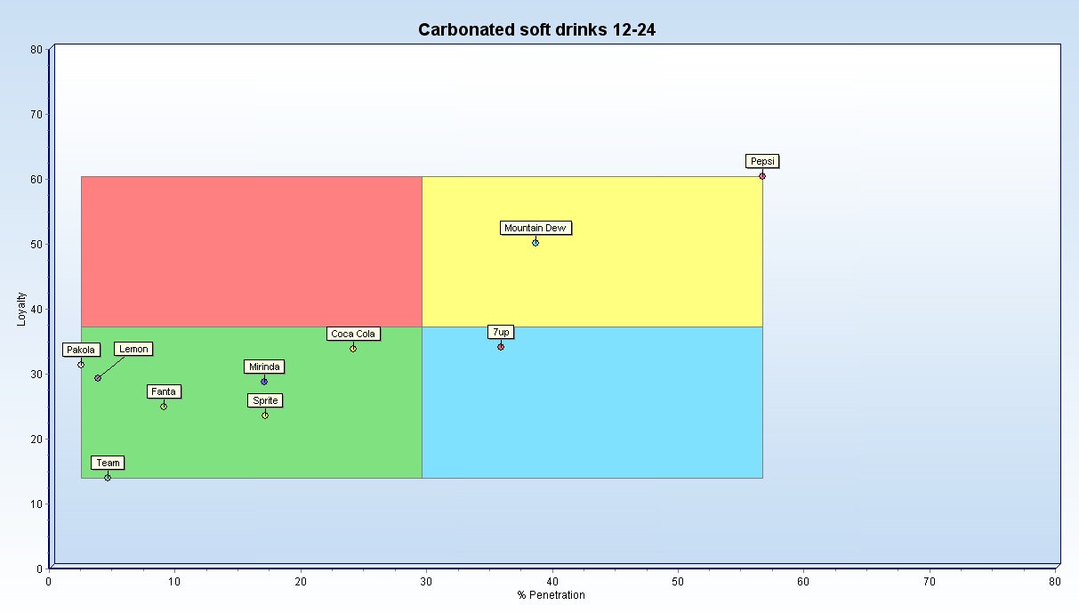
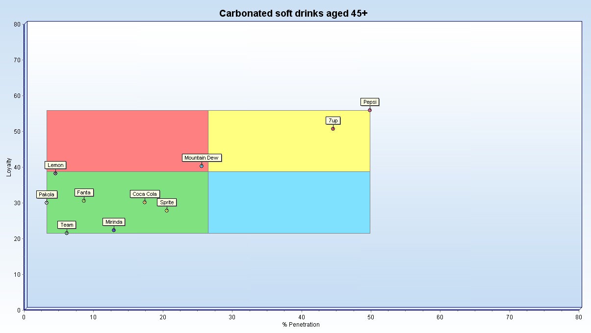
The two charts above contrast visually the market structure and brand positions for carbonated soft drinks between the younger
(10.3m. 12-24’s) and the older (5.3m 45+). In the younger group the (any usage) penetration is considerably higher (56%) and the loyalty level by brand is more spread (15-60%). While Pepsi is the leading brand in both groups in terms of both penetration and loyalty in the older group it is closely followed by 7up with Mountain Dew in third place with much lower penetration and only an average level of loyalty. In the 12-24 group it is Mountain Dew that moves up ahead of 7up and closer to Pepsi.
Annex 3 – The socio-cultural segmentation Segment 1 Traditionalist (14.7%)
 Satisfied & safe, Religious and spiritual, status quo, digitally cautious, order & planning
Segment 2 Fantasists (13.8%)
 Uncertainty, salary = success, fashion & prestige, enjoyment/convenience
Segment 3 Star Plused (15.4%)
 Stay at home moms, love Indian dramas, celebrate events, non technology
Segment 4 Sci Fi’s (16.5%)
 Young & agile, knowledge driven, ready to change, fast moving, heavy media consumers
 Segment 5 Necessitous (11.9%)
The have nots, low education/illiterate, limited media exposure
 Segment 6 Householders (15.5%)
Domestics, gossipers, like commercials, use ready to cook and recipes, responds Direct
Marketing
Segment 7 Off Road Consumers (12.3%)
 Social outcaste, indecisive, hard to convince/influence, un-opinionated
This segmentation has proved to be very discriminatory in terms of product and brand usage and ownership as the following table indicates.
| Items Owned At Home | ||||||||
| Base pop | Vacuum
Cleaner |
Hi-Fi | Elec kettle | Dish
washing/m |
PC | Mobile | Radio | |
| ‘000 %^ | %> Idx | %> Idx | %> Idx | %> Idx | %> Idx | %> Idx | %> Idx | |
| Traditionalists Fantasists Star Plused
Si-Fi’s Necessitious Householders Off Road Commuters |
4186 14.7
3922 13.8 4390 15.4 4697 16.5 3401 11.9 4410 15.5 3498 12.3 |
2.7 118
2.2 93 1.3 58 4.9 211 1.1 46 1.8 76 1.7 74 |
4.4 200
2 92 1.8 80 3.5 157 0.5 24 1.5 66 1.2 55 |
7.2 252
2 71 1.7 60 3.5 124 1.1 38 2 71 1.9 65 |
2.7 82
4 121 2.2 67 6.3 194 1.5 47 2.1 63 3.6 112 |
14.9 141
7.8 74 8.5 80 17.4 165 6.6 62 9.6 91 6.9 66 |
76 108
69 98 69.9 100 79 113 58.4 83 71.5 102 62.8 90 |
9.7 121
6.1 76 7.4 92 11 137 5.6 69 6.3 79 9.5 119 |
| Total | 28504 100 | 2.3 100 | 2.2 100 | 2.9 100 | 3.3 100 | 10.6 100 | 70.2 100 | 8 100 |
Notable is the extremely low homes penetration of durables including radio sets with the exception of mobiles which is over 70% and the importance of Sci-fi’s and Traditionalist for these markets.
Annex 4 Feeling and activities – some results
One of the reasons behind these questions was to see if there was evidence of a general anger or depression s a results of the constant power outages that have been crippling the Pakistan economy over the last 18 months. It is however difficult to see the effects in the data as the outages are fairly random and could last more the 24hrs in some places, so regional and time differences are obscured and, as they have been going on for so long, people have had to come to accept and live with them.
| At Home, Net share % of all feelings Preoccupied,Stressed,Angry,Depressed Happy,Calm/Relaxed
Tired,Bored At Work, Net share % of all feelings Preoccupied,Stressed,Angry,Depressed Happy,Calm/Relaxed Tired,Bored Travelling, Net share % of all feelings Preoccupied,Stressed,Angry,Depressed Happy,Calm/Relaxed Tired,Bored At place of prayer, Net share % feelings Preoccupied,Stressed,Angry,Depressed Happy,Calm/Relaxed Tired,Bored |
Av day by time, those in employment (11.2m) | ||||
| 07:00-
08:00 |
12:00-
13:00 |
16:00-
17:00 |
19:00-
20:00 |
22:00-
23:00 |
|
| 7.8
89.5 2.6 13.3 83.7 3 11.8 80.7 7.5 6.9 93.1 0 |
19.1
70.1 10.8 23.5 67.3 9.2 27.5 56.5 16 14.6 61.4 24 |
13.6
75.5 10.9 22.2 63.4 14.4 18.5 52.7 28.8 19.1 64.9 16 |
13.1
75.1 11.7 16.1 69.6 14.3 16.5 60.3 23.2 14.3 72.1 13.6 |
5.5
86.3 8.2 12.3 72.6 15.2 12 67.8 20.1 2.9 91.4 5.7 |
|
Amongst those in employment the high happy and calm levels of the early morning (especially while at prayer) drop considerably during the day even while at home and while praying but are restored by 22.00. Stress level rise sharply by lunch time at work and particularly while traveling but recede in the afternoon and evening being largely replaced (especially while travelling) by boredom and tiredness.
Annex 5 – VDiary results for selected vehicles compared with the ‘Recency’ control at day and week level by key demographics
| Newspapers | All pop | Age 12-24 | SEC A1,A2,B | |||
| Sample/prfl | 10038 | 100 | 3608 | 35.9 | 3986 | 39.7 |
| Pop 000/prfl | 28504 | 100 | 10328 | 36.2 | 7938 | 27.8 |
| 000 | Week | Av Day | Week | Av Day | Week | Av Day |
| Dawn VDiary | 440 | 192 | 180 | 77 | 331 | 142 |
| Dawn ‘Recency’ | 440 | 192 | 180 | 73 | 331 | 145 |
| Express VDiary | 2227 | 1143 | 821 | 404 | 870 | 457 |
| Express ‘Recency’ | 2230 | 1140 | 821 | 378 | 871 | 467 |
| Khabrien VDiary | 807 | 353 | 244 | 99 | 255 | 113 |
| Khabrien ‘Recency’ | 807 | 354 | 244 | 85 | 255 | 103 |
| Nawa I Waqt VDiary | 1391 | 648 | 347 | 145 | 548 | 268 |
| Nawa I Waqt ‘Recency’ | 1392 | 646 | 348 | 127 | 548 | 294 |
| Television | All pop | Age 12-24 | SEC A1,A2,B | |||
| Sample/prfl | 10038 | 100 | 3608 | 35.9 | 3986 | 39.7 |
| Pop 000/prfl | 28504 | 100 | 10328 | 36.2 | 7938 | 27.8 |
| 000 | Week | Av Day | Week | Av Day | Week | Av Day |
| Cartoon Network Vdiary | 2558 | 1667 | 1410 | 934 | 765 | 490 |
| Cartoon Network Recency | 2558 | 1646 | 1410 | 952 | 765 | 510 |
| Geo Entertainment Vdiary | 1842 | 1043 | 755 | 403 | 677 | 379 |
| Geo Entertainment Recency | 1858 | 1039 | 755 | 407 | 680 | 417 |
| PTVhome Vdiary | 3939 | 2530 | 1549 | 1015 | 971 | 592 |
| PTVhome Recency | 3942 | 2519 | 1552 | 1030 | 972 | 611 |
| Sony Vdiary | 3222 | 1509 | 1379 | 649 | 890 | 406 |
| Sony Recency | 3221 | 1484 | 1378 | 658 | 890 | 407 |
| Radio | All pop | Age 12-24 | SEC A1,A2,B | |||
| Sample/prfl | 10038 | 100 | 3608 | 35.9 | 3986 | 39.7 |
| Pop 000/prfl | 28504 | 100 | 10328 | 36.2 | 7938 | 27.8 |
| 000 | Week | Av Day | Week | Av Day | Week | Av Day |
| Fm 101 VDiary | 737 | 414 | 451 | 267 | 231 | 134 |
| Fm 101 ‘Recency’ | 737 | 407 | 451 | 269 | 231 | 134 |
| Fm 103 VDiary | 790 | 466 | 487 | 286 | 207 | 130 |
| FM 103 ‘Recency’ | 790 | 464 | 487 | 285 | 207 | 140 |
| Fm 106.2 VDiary | 633 | 384 | 421 | 251 | 245 | 150 |
| Fm 106.2 ‘Recency’ | 633 | 381 | 421 | 246 | 245 | 139 |
| Fm 107 VDiary | 397 | 239 | 276 | 177 | 136 | 92 |
| Fm 107 ‘Recency’ | 397 | 240 | 276 | 176 | 136 | 106 |
| Internet | All pop | Age 12-24 | SEC A1,A2,B | |||
| Sample/prfl | 10038 | 100 | 3608 | 35.9 | 3986 | 39.7 |
| Pop 000/prfl | 28504 | 100 | 10328 | 36.2 | 7938 | 27.8 |
| 000 | Week | Av Day | Week | Av Day | Week | Av Day |
| Yahoo Vdiary | 855 | 480 | 495 | 280 | 549 | 315 |
| Yahoo Recency | 855 | 478 | 495 | 274 | 549 | 301 |
| Gmail Vdiary | 141 | 87 | 72 | 47 | 92 | 60 |
| Gmail Recency | 141 | 91 | 72 | 46 | 92 | 62 |
| Hotmail Vdiary | 354 | 208 | 220 | 138 | 262 | 154 |
| Hotmail Recency | 354 | 207 | 220 | 149 | 262 | 157 |
| Google Vdiary | 679 | 388 | 421 | 244 | 446 | 264 |
| Google Recency | 679 | 388 | 421 | 238 | 446 | 268 |