François Charton and Antoine Taconet, Carthage & CMBS

Worldwide Readership Research Symposium Valencia 2009 Session 5.2

The scope

Most Media planning models work under the assumption that one opportunity to see is delivered with every exposure, and that those OTS can be freely added to.

This model has proved very efficient as long as it was used within one media, and as long as the definition of “exposures” was chosen to fit its prerequisite. However, it has limitations, and it does not permit us to make full use of different measurements of audience.

In print, it cannot take into account

• The fact that only a part of a magazine is read (therefore lowering the actual reach)
• The number of times the same magazine is read, or the number of pages read, (which would increase the GRPs)
• The time spent reading a magazine

For Internet, three indicators are typically measured. The unique visitors per day, which tend to be used as probabilities, the number of pages viewed (which are what media planners buy) and, or a time spent on a website. In addition, a website is often partially bought (as a global number of pages, as a share of voice, or through capping).

These aspects do not fit easily into classic Media planning models. At a time when we want global reach estimates for print + internet, it is a pity.

For Radio and TV, probabilistic models do not distinguish between persons who visit every other day and listen to/watch the whole break and people who visit every day and watch half of the break. Factors like the duration of viewing over a period, and the number of different channels watched are not taken into account. Finally, twin spots (two ads for the same product in a break/period) are not correctly counted by many models.

On cross-media models, the assumption that opportunities to see can be freely added to does not hold (partly because measurement methodologies and definitions of contact vary from one media to the other)

In this paper, we will propose a new model, the fractional binomial model, derived from formal calculus, which can handle all such cases, and therefore is more generally useful than all previously known Media planning models.

In this model, individual exposures to a media plan are represented by polynomials. Simple operations, like adding or removing one insertion to a plan, merging two plans together, or calculating reach, GRPs or frequency, translate into basic algebraic operations, which can accommodate many different situations.

We will also show that this approach is not contradictory to efficient calculations.

Also, such models are amenable to faster calculation, using Laplace and Fourier transforms, which opens new opportunities for optimisation tools.

Key words

Media planning, probabilities, share of voice, models, transforms, polynomials, quick calculations

The use of probabilities versus models

Most media planning tools belong to one of two categories.

Probabilistic tools calculate, from audience surveys, individual probabilities of contact between respondents and media, and aggregate respondent level models of exposures, over various target groups.

Model based tools use, for each target group, a series of aggregated formulae (adjusted to audience results), which calculate reach and frequency distribution, from duplication matrixes measures from the data.

We do not wish to enter the “religious” quarrel of the value of each method.

We have used both and recognize their respective merits and drawbacks. However, we think that all model approaches can be approximated by probabilities, given a correct choice of the underlying distribution. For instance, the Metheringham model can be shown to be equivalent to individual probabilities from a beta distribution.

More generally, a theorem by Hausdorff (studied, by De Finetti, and more recently by Diaconis) shows that under relatively sensible assumptions (diminishing returns on the cumulative reach increase) any formula can be matched with an underlying smooth probability distribution. But this is not our topic for today.

Here, we work on probabilistic approaches, for two reasons.

• As the number of vehicles grows, the calculations of duplications will rapidly grow and might reach a limit.
  • A print survey has hundreds of titles.
  • A radio survey may have as many as 50 stations, 3 types of days and 96 ¼ hours, thus a few thousand vehicles.
  • A typical Internet survey also consists of a few thousand vehicles.
  • A TV survey may handle 50-250 stations, 7 days and 96 ¼ hours meaning as many as 150,000 vehicles (using average days and not dates).
  • The calculation of duplications in the case of a small TV survey with 100 stations thus represents a duplication matrix with more than a billion cells.
• There is an increased demand for cross-media planning, where probabilistic approaches seem better adapted.

The classic probability approach

Here are a few words to remind the readers of the assumptions and mechanisms behind this approach.

Probabilistic methods consider that, for each respondent i and for every media vehicle v (note: media vehicles are the building blocks of media planning, their nature changes from one media to another: in print, they will usually correspond to one average issue of a magazine, in internet to one website over a day, in radio to a ¼ hour, or a half hour period, over one day, …), a probability of being exposed p_iv can be calculated.

Those individual probabilities are then fed into a model, which assumes that exposure to different vehicles (or to the same vehicle on different days/issues) are statistically independent (this specific model is know in literature as binomial, or full binomial). For a given media plan, the probability that a specific respondent is exposed k times can be derived from the probabilities.

For instance, if the respondent is exposed

• To vehicle 1 with probability p (example p=0.2)
• To vehicle 2 with probability q (example q=0.4)

For a plan with 1 insertion in each vehicle, they will be

• Exposed 0 times with probability (1-p)(1-q) ➔ 0.48
• Exposed 1 time with probability p+q-2pq ➔ 0.44 totaling 1
• Exposed 2 times with probability pq ➔ 0.08

If a third insertion is added, for which the probability is r (example r=0.7), the respondent will be

• Exposed 0 times with probability (1-p)(1-q)(1-r) ➔ 0.144
• Exposed 1 time with probability p+q+r-2pq-2qr-2rp+pqr ➔ 0.468
• totaling 1
• Exposed 2 times with probability (pq+rp+qr-3pqr) ➔ 0.332
• Exposed 3 times with probability pqr ➔ 0.056

For a media plan, such calculations are done at the individual level, adding insertions one by one.

Let P(n,k) be the probability of being exposed k times after the n^th insertion (the order of the insertions is irrelevant to the result), we have

P(0,0)=1

P(0,k)=0 for k>0 (i.e. the individual is not exposed)

And if insertion n has probability r P(n,0)=P(n-1,0) (1-r)

P(n,k)=P(n-1,k)(1-r)+P(n-1,k-1) r (k>0)

The calculations behind that approach are formally equivalent to polynomial multiplications. Let us denote q= 1-r the probability of respondent i not being reached by vehicle v, and writing P_n(X)= P(n,n) Xⁿ + P(n,n-1) X^n-1 + … + P(n,k) X^k + … + P(n,0)

We have P_n(X)= (q+rX)P_n-1 (X)

Or in a more formal writing, if one has several vehicles: (1)

v v

Nv

((1 p )  p X )



vlist

Or even more formally: (2)

((1 p)  pX )N

Such calculations are performed at the individual level, and the results need to be summed for all respondents in a target group, to provide the reach and frequency distribution of the plan.

The polynomial representation is strictly equivalent to the usual methods we use for probability models, but it can help in different ways.

It simplifies many calculations. Suppose we have calculated individual probability of exposures for two different plans, and let P(X) and Q(X) be the corresponding polynomials. The exposure distribution of the global plan is the product P(X).Q(X).

Conversely, removing a “sub plan” from a plan can be done easily by dividing the corresponding polynomial (in increasing order of powers, in practice, polynomials will be truncated to the degree corresponding to the highest reach we want to measure).

When working on large plans (in optimization notably), such multiplication formulae speed up calculations.

Also, it allows for a good description of packages. For instance, a group of magazines bought together as a package (or a set of promotional screenings around a sports program) can be represented, inside a Media planning model, as a specific polynomial.

Finally, calculations on polynomials are a heavily researched mathematical subject, one where many efficient techniques can be used. To give one example, calculations involving many polynomial products can be sped up by techniques using Laplace or Fourier Transforms. Such methods can therefore be efficiently used for optimizers.

The advantages and drawbacks of this approach

The probabilistic approach is well known and has given rise to many robust implementations for the benefit of the advertising world.

However, it takes in to account a simple answer to a straight question such as

• • “Have you read or looked into a copy of the publication in the last publication period?”
  • “Were you listening to this radio station between 700am and 715am yesterday for at least 1 minute?”

And the paradigm is that for each person saying ‘yes’ one, and only one, contact is delivered. The probabilities that are derived work on the same assumption.

However the surveys of today are a lot richer and the reality of buying has changed.

The new questions to be taken into account

• Most of the print surveys these days have one or several questions, and information is taken from this (non exclusive) list (either asked directly, or derived from another set of indirect questions):

1. How long do you spend reading this magazine or daily?
2. How many pages on average do you read?
3. How many issues of the title have you come across?
4. How many times have you had this particular copy in hand?

We have moved far from the simple question (“Have you read or looked at a copy of the publication in the last period?”) which in our country used to read “Have you read, flicked through or even had a glance at this particular publication” so keen were the editors to count as many readers as possible (that was a long time ago though).

• • In the Internet surveys made with panels, not only a daily contact is measured, but also a number of pages and a time spent (not taking into account the time of the day when the contact takes place). There is a need to take those numbers of pages into account. It is all the more true if one (there is a big demand for it) wants to have results on

combinations of media such as Print

+ Internet.

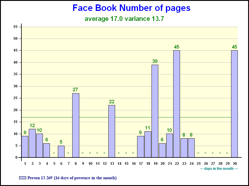
The graph shows the daily number of pages for a person present 16 days during the month

• The radio surveys measure whether a person has been in contact with one or several stations in the same quarter hour. Also, some attempts have been made to measure radio pretty much the same way that TV is measured.
• TV panels measure a number of seconds in which a person was present during a break. Should all persons be equal, or are other means required?

The reality of buying

The way advertising is bought is changing. This is especially true for Internet, but we will see that also Media planning on traditional media could reflect the reality of buying more precisely:

A web surfer may be in contact with 17 pages of Face Book on an average day. Does it mean he (or she) has 17 contacts (on average) when they surf on this site?

Obviously no, for two reasons

• One is that 17 is an average and the detail is as given on the previous slide (however ,this might only be a small problem or even a problem at the individual level and not on the whole)
• The other reason is that an advertiser does not buy the whole of a site but only a {small} portion. We will call that the share of voice. For the sake of our example, let us imagine the advertiser has bought 1/1,000^th of the site which might even be an exaggeration in this case.

What can we do with the three new figures that we have?

• the 17 pages on an average day
• the variance of 13.7
• the share of voice of 1/1,000^th

Does it mean that our person sees 0.017 pages?

In this case we understand how this could contribute to GRP calculations, but how could it play a role in the distribution of contacts? More about this later.

Other situations are not so easy to cope with.

How to evaluate a plan with twin spots (30”+8”) in the same break?

How to evaluate a plan which contains twin spots (30”+8”) in the same break, as well as 30” spots? How to compare plans with 20” spots with plans that have 30” spots?

The problem is the same for print with many different formats, not to mention Internet and all its exotic formats.

Finally, the trickiest problem of all, which in most markets is almost a religious issue,: how to add up the apples and the pears, meaning how to evaluate a plan with two different media when all the editors and vested interests swear their media is really unique.

What is our suggested solution?

We are proposing both a formal solution derived from the polynomial formalism, coupled with a practical application.

A new probabilistic approach

As we have seen, the polynomial formalism represents exposure at the individual level as polynomials.

As often with polynomials, it seems at first glance that the variable, X, has no practical significance. Or has it?

We propose to make use of the variable X, or rather, to replace it with others, in order to incorporate new elements to the binomial model.

How much is an exposure? The case of twin inserts, and page views…

The polynomial representation offers a very simple solution for twin spots. For those insertions, replace X with X²… The polynomial is now (1-p) + pX² which means the individual has a probability p of seeing both of the ads.

This could be further generalized if some information is available about the number of pages read in a magazine, (or pages viewed on a website). Such information is available in some audience surveys. At the individual level, X can then be replaced by another polynomial, which describes the number of contacts for each visit.

For a magazine, suppose the audience survey measures the number of reads of an issue, and concludes that a given respondent reads, on average, the magazine twice. A first approximation could be to replace X by X², or, even, X^2.3, but if more precise information is available, we might use a more complex polynomial, like 0.2 X + 0.6 X² + 0.2 X³ which would quantify, in the Media planning evaluation, the fact that on average readers read the magazine once 20% of the time, twice 60% and three times 20%…

Using such techniques, we can derive frequency distributions for print or internet, not only in terms of visits or issues read, but also in terms of page views.

A similar approach could be used in order to tackle the viewing duration of a media… (seconds, or minutes, replacing pages)

Having our cake and eating it… Multimedia, multi-criterion

Polynomial representation solves this problem by using different variables for different media (or criteria).

For instance, in a Print+Internet survey, we may have, for a respondent, both their probability of reading a magazine, and their probability of visiting a website. Using the polynomial representation, we can carry out both calculations at the same time, provided we use different variables for different media (say X for print, Y for internet).

In the end, we get a bivariate polynomial Q(X,Y), which gives the probability of being reached by both media… This allows for the calculation of joint exposure distribution, from single source or fused surveys, whilst still using the tradition Media planning tools (and, therefore, staying consistent with existing market standards).

Equally, we could evaluate a monomedia plan on two different criteria, say an internet plan on pages and duration… Just replace the X with a polynomial in P(age) and T(ime), which gives the average time and page views for each visit (this is available from audience surveys).

Bits and pieces – Partial reads, Partial buys

One last challenge, which sometimes arises, is taking into account partial reads of a magazine, or, on the internet, partial buys of a website (the so called “share of voice” concept above, where one’s ad can be displayed on 10% of the available pages, selected at random).

Again, the polynomial model can solve this by replacing the variable X with another one which takes the partial reading into account. If, for instance, only 25% of the magazine was read (or 1/4 of the break was watched, or 25% of the website was bought), X can be replaced with 0.75 + 025 X.

Stretching the formalism

Incorporating the three changes described above,

1. can be rewritten

((1 p)  pX ^ )N .((1 q)  qY ^ )M

((1 p)  pX )N

• X and Y stand for two different media

1. where

•  &  stand for the effect of the contact. It might as well, at this stage, represent both the number of pages and the variance or only the average.  might be an integer or a real number (as far as the formalism is concerned this is not a real problem).
• N & M represent the number of insertions in the vehicle.

In the development of the polynom, the term in X^k Y^m represent the portion reached k times by the medium corresponding to X and m times by that corresponding to Y.

How shall we cope with the share of voice?

We feel that this has to be treated with a change in variable. Suppose that we buy 1/1,000^th of the pages of a site, a person visiting a page of the site has a probability of 1/1,000^th to be reached and a probability of 1-s of not being reached. We ignore here, superbly, the fact that that the site may target the persons and therefore play on the probability, which means that the share of voice can or should be translated at the individual level, but that leaves some food for thought for the coming years.

Therefore in this case X corresponds to ((1-s) + sX) and X^k corresponds to ((1-s) + sX)^k.

The formula becomes

((1 p)  p((1 s)  sX )^ )N .((1 q)  q((1 t)  tY )^ )M

What are the different levels?

((1 p)  p((1 s)  sX )^ )N

For one medium only:

For each person and each vehicle we have:

• The probability of being there one day (➔p).
• The level of consumption (number of pages + if necessary the variance➔).
• (note for print we might have here the proportion of issue read ➔s) For a given plan for each vehicle we have:
• The number of insertions (➔N)
• The share of voice (➔s) Naturally, when s=1 the above formula becomes

((1 p)  pX ^ )N

(5).

(4).

And if =1 it simplifies anew into

((1 p)  pX ^ )N

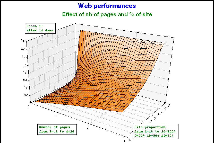
How can we make good use of it?

the original formula

This would be another piece of “scientific talk” if, in parallel, we had not developed a tool that translates this formalism into reality and which therefore allows our users to

• Use the combination of Print + Internet
• Make good use of the number of pages visited on the Internet
• Translate the share of voice and allow for a realistic evaluation
• Eventually incorporate new measurements of print, when they are ready (or complete)

Our calculations respect the three following rules

• Rule number 1: The reach of the plan must be equal to the value given in the following formula.

(1 (1 p((1 s)  sX )^ )N )

The reach is

 (1 (1 p)N )

or

And that is defined whether N and  are integers or real numbers

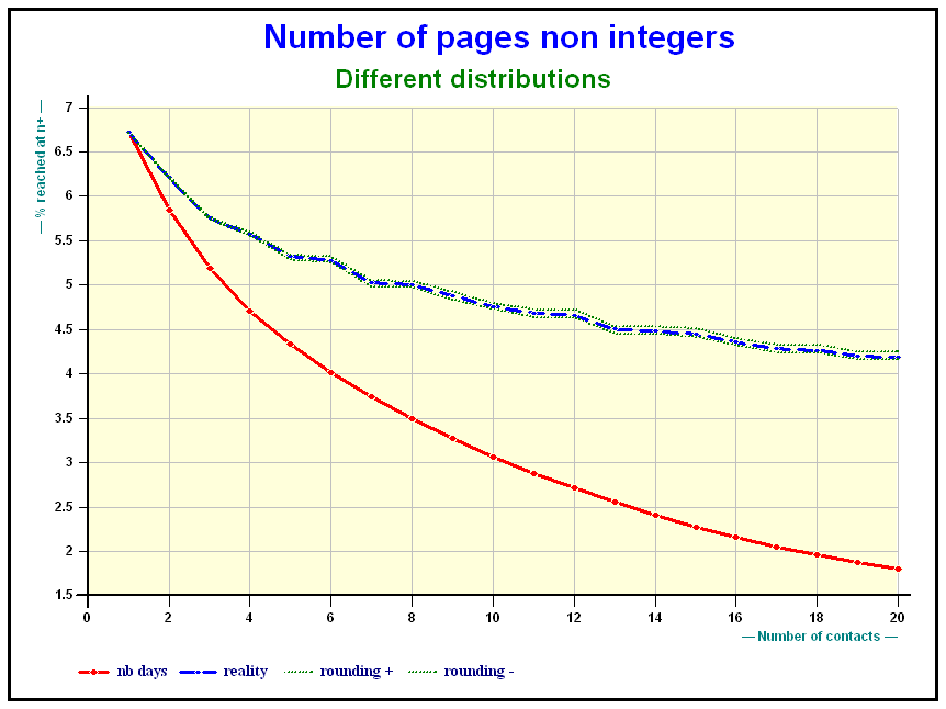
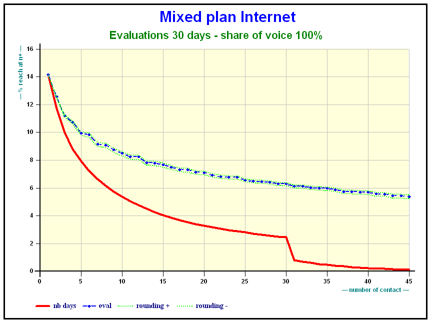
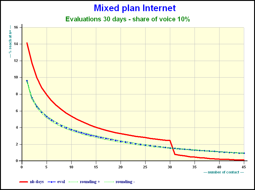
• Rule number 2: The Cumulative distribution must be comprised between that obtained by rounding up the  and that obtained by rounding them down (see slide)

• Rule number 3: There must be a continuity, both in terms of variables or target groups, and in terms of ’s (and in the future of N, if one wants to consider that).

In addition, we have conducted a number of tests which have allowed us to determine what type of action is to be taken. In other words, where the situations are when the calculations must use all of the distribution of the number of pages seen on the Internet, and when an average and a variance is sufficient. This is so that the calculations are kept fast enough for tools to use efficiently.

What are the results?

All the examples taken here are taken from an Official Print survey (AEPM with a sample of more than 21,000 persons of which of which 15,000 use the Internet) “coupled” with an official Internet survey (NNR with a sample of more than 15,000 persons) .

The coupling is a simplified form of fusion, but the effects of the different results are preserved.

Nevertheless the number of issues were only available for the yesterday readers and we have taken the hypothesis (quite unproven and risky, but not totally absurd) that all the readers would follow the same pattern. And the proportion of reading has also been partially made.

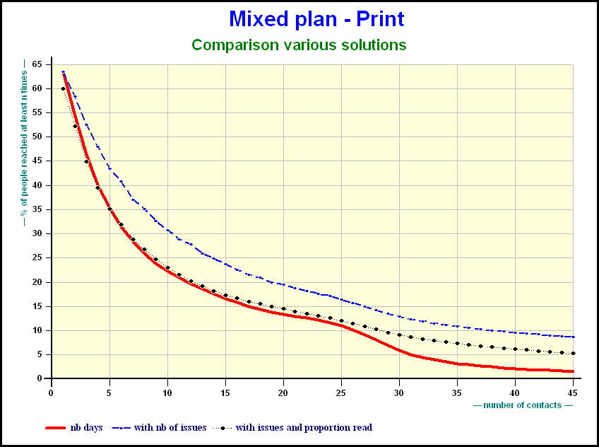
The number of issues amplifies the results for the titles:

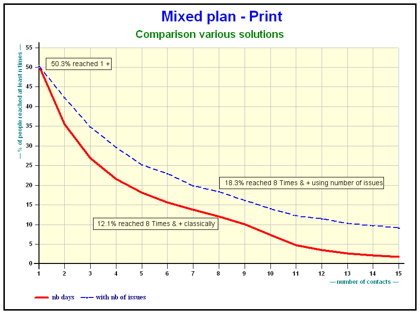
This slide as well as the following slides illustrate cumulative reach of a plan using different methods. The combination of the number of issues plus proportion read, more or less, compensate one another. The reach diminishes. The queue of the distribution is higher.

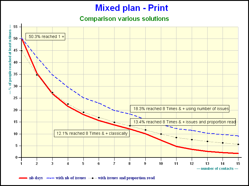
When the number of days grows the gap in reach is smaller.

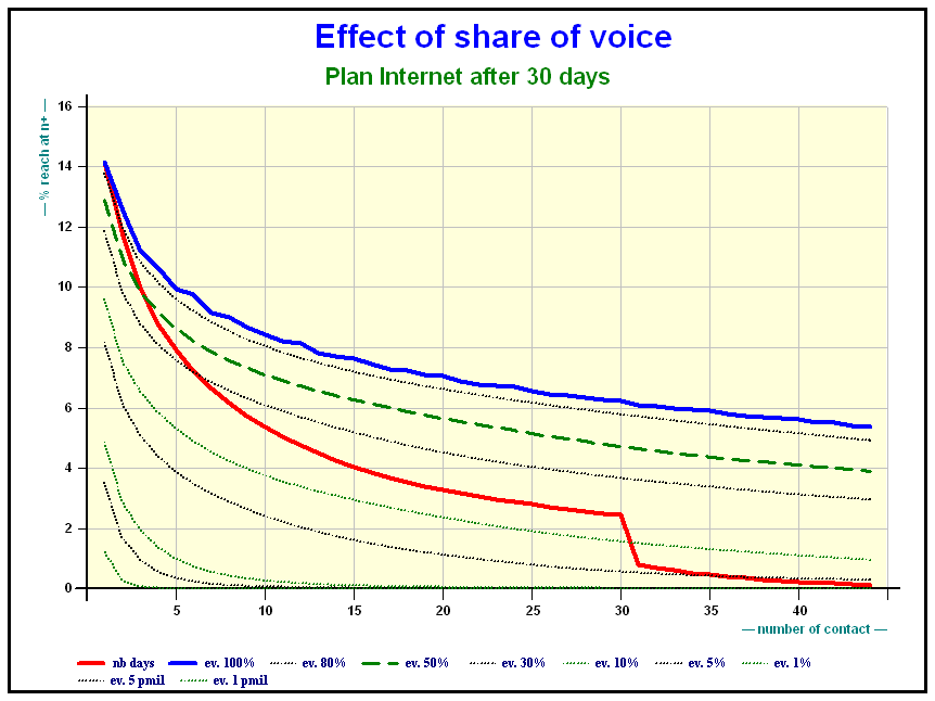
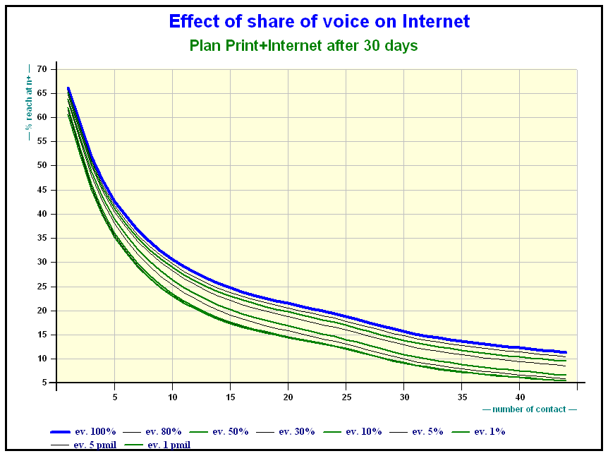
As far as Internet is concerned the effect of share of voice is obvious.

Here is the effect of the share of voice on a mixed Internet plan after 30 days

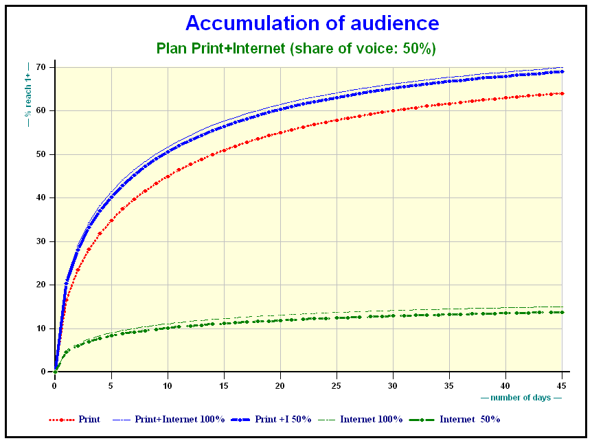
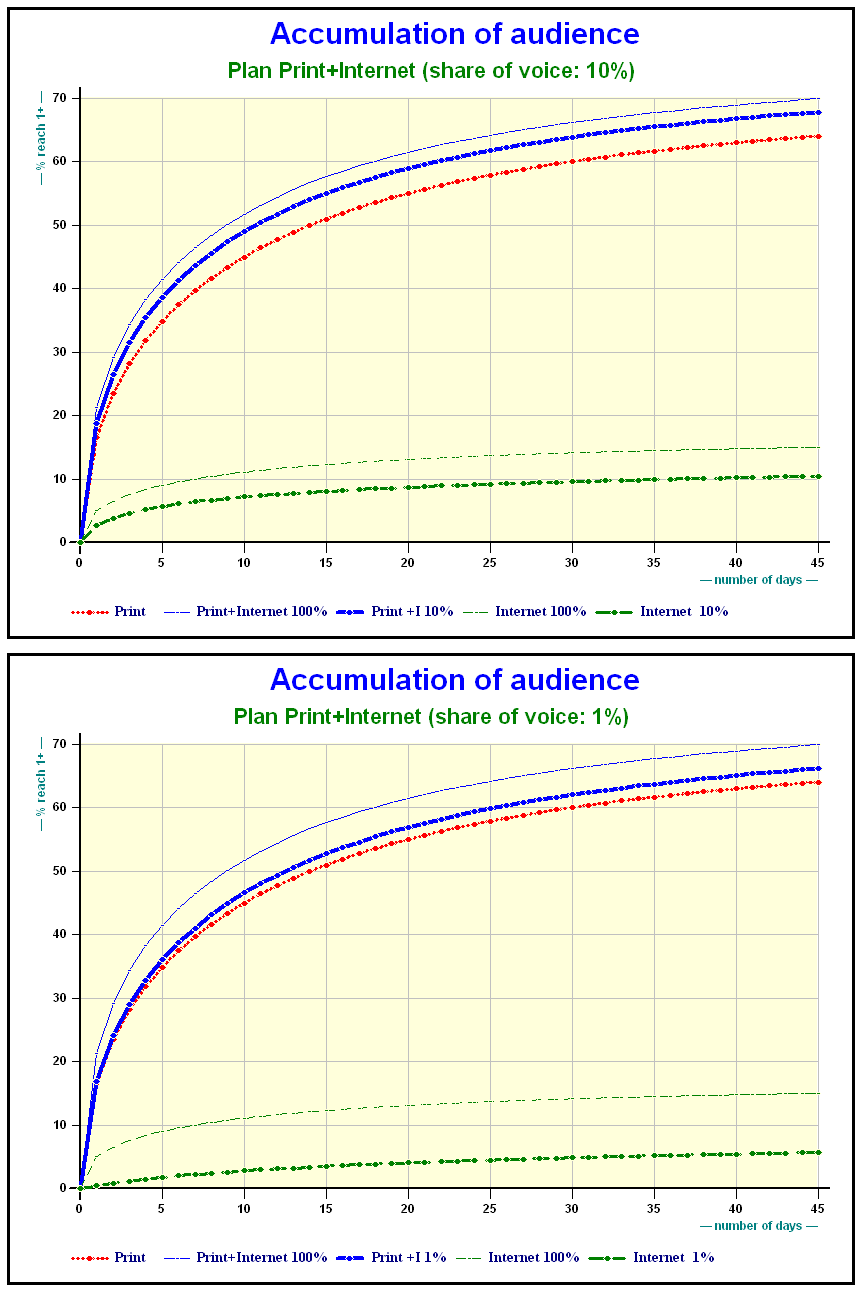
Results on Print + Internet

Accumulation of audience Print + Internet plans

When should this method be used?

Since it generalizes the binomial method, the fractional model can be used in the same situations: media planning, or mixed media evaluation.

It is meant to use additional data, page views, cross media surveys, or other indicators, which may be provided by the same survey, or via separate research.

For print

• It should be used
  • when number of pages are available per person
  • and (even better) when on top of that a proportion of reading (at the individual level) or a share of voice (at the level of the plan) can be taken into account.
• It can also be used
  • If the number of pages per group of people is available after one has made sure that the results are not too distorted. When thinking about the numerous publications where print is available with details and Internet is also available but only at the day level there are at least two methods worth considering:
    • The fusion of data with the import of pages per person
    • The import of results per target group (probably after a CHAID analysis). This method has to be proved robust and one has to check whether original results are preserved, but it is a way that deserves to be explored further.

Conclusion

In this paper, we have described a formalism, and shown a number of possible applications. However, research on such algebraic models is ongoing, and will certainly provide new ideas and insights with time.

There are two potential uses of such fractional models:

• First, the polynomial formalism links media planning calculations to a heavily researched field of mathematics (polynomials, power series, and their use in fast computation). In the long run, it means both a better understanding of the theoretical aspects of the models we use, and better computation of the models.
• Second, they provide a framework for incorporating new data (apart from exposure) into media planning models.

As such, the existence of such models should encourage the development of new measurement approaches to media.